WHITEPAPERS
Signal Processing in Manufacturing Applications – an Engineer’s Guide
In this whitepaper, we’ll discuss common sources of noise in industrial environments that your engineering team is likely to encounter. We’ll also provide a few standard and advanced signal processing techniques to help you get started.
Executive Brief
In manufacturing, being able to create, price and distribute products as efficiently as possible is critical to profitability. Data science has become a powerful tool to accomplish this, particularly when paired with machine learning. While these technologies are impressive, they’re also complex and full of risk for those who aren’t yet experts in applying them.
Machine learning models in manufacturing applications often rely on data provided by sensors, and sensors in production environments are imperfect devices. Because of their smaller size, they sacrifice signal or measurement quality compared to more expensive laboratory-grade equipment.
So, how do you avoid being caught in a “garbage in, garbage out” situation? Using the signal processing techniques listed in this whitepaper, your engineering team will be able to identify sources of noise in your system, refine the data, and reveal the actual signal coming from your systems. You can feed this refined signal data into machine learning models applied to predictive maintenance, quality control, forecasting, process control and optimization, and more.
Introduction
As more and more devices generate more data at increasing levels of sensitivity, noise becomes a major factor that can interfere with the data collected by your sensors. How do you determine the valuable information and ignore the distracting noise? Signal processing, as a discipline, solves this problem. Since industrial environments generate a lot of noise, signal processing has become an integral part of the Industry 4.0 landscape.
In this whitepaper, we’ll discuss common sources of noise in industrial environments that your engineering team is likely to encounter. We’ll also provide a few standard and advanced signal processing techniques to help you get started.
The Evolution of Sensors in Industry
Industrial settings measurements have come a long way since the First Industrial Revolution. Industry has evolved from manually monitoring steam-powered processes to using hundreds of thousands of advanced electronic sensors — devices that measure or detect a physical property — to measure complex physical phenomena.
These sensors first became an integral part of industry in the 1970s during the Third Industrial Revolution, where processes began adopting programmable memory controllers and started making their processes autonomous.
As time passed, sensors became smaller, cheaper, and capable of capturing physical properties beyond pressure, temperature, and volume. These newer, more advanced sensors can capture spectral information in more than one dimension as well as render three-dimensional space using technology such as LiDAR. Coupled with the advancement of networking, cloud infrastructure, and big data, Industry 4.0 has arrived.
Industry 4.0 combines the internet of things (IoT), cloud computing, analytics, and machine learning to automate and digitize manufacturing-related industries. These combined technologies provide more accurate information about the real-time environment, allowing businesses to shorten the feedback loop and improve their decision making.
Industry 4.0 combines the internet of things, cloud computing, analytics, and machine learning to automate and digitize manufacturing-related industries.
Choosing Sensors: Size vs. Signal Quality vs. Measurement Speed
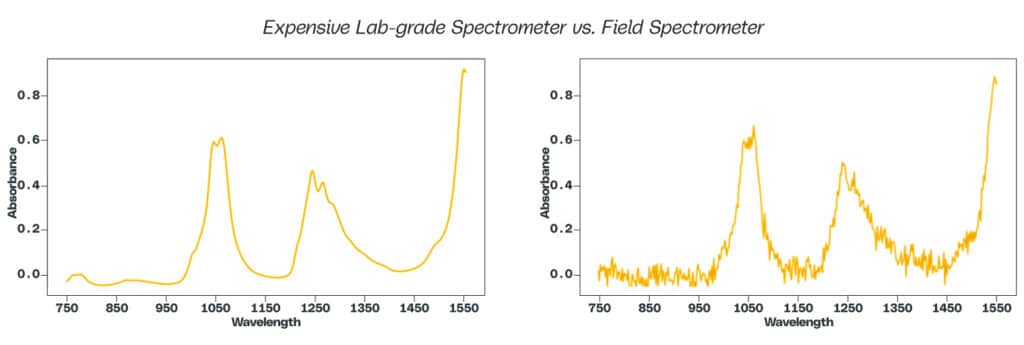
While the technology is impressive, it has limitations. Sensors in production environments are imperfect devices. Because of their smaller size, they sacrifice signal or measurement quality compared to laboratory-grade equipment that measures the same phenomena. To illustrate this point, here are two spectra measuring the near-infrared absorbance of the same diesel fuel sample, which is useful for automating diesel and gasoline blending in refineries. The spectrum on the left clearly has a more well-defined shape than the spectrum on the right, which appears noisy, because the spectrum on the left was obtained using an expensive laboratory-grade spectrometer, whereas the spectrum on the right was obtained using a field spectrometer.
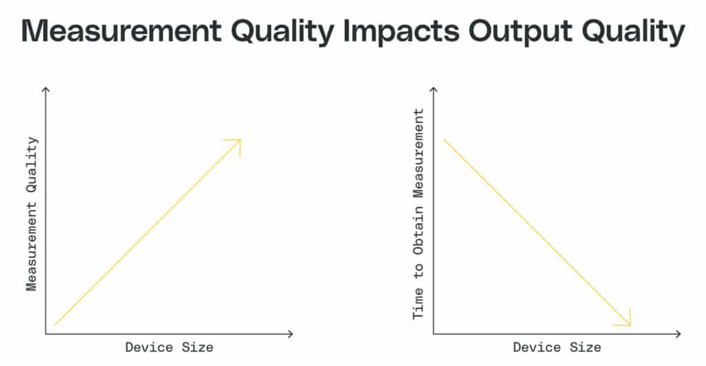
Measurement quality correlates proportionally with sensor size — as sensors become larger and more expensive, measurement quality improves.
This quality difference leads to an important correlation between sensor size, measurement quality, and timeliness. When it comes to the installation of these sensors in industrial facilities, size matters. As sensors shrink, they can be installed into a greater range of production environments — often even inside production machinery. This allows for faster measurement. In other words, the time to obtain a measurement is inversely proportional to its size.
We need to understand these relationships because they will help us choose the right type of sensor for your particular application.
Measurement quality leads to data science and machine learning output quality as well. In some cases, we will not use a direct sensor reading to measure process behavior or quality directly. Instead, we will use the reading as part of a calculation or model to infer another value. As a result, measurement quality can have a significant impact on calculated outputs. For example, as shown below, two models trained from a field sensor and a laboratory sensor on the same set of samples can have different outputs in predictive capability.
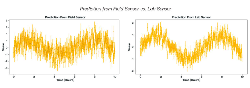
The error bars and range in prediction can be substantial when comparing a field sensor with its laboratory counterpart.
While we might get measurements quicker, there is a tradeoff in measurement quality that can have downstream consequences. To accommodate this tradeoff, we must understand the fundamental concepts around sensors, signal, noise, and signal processing techniques.
What Is Noise and Why Does It Matter?
Sensor output values include the measure of a physical property, but they also include extra values. Sensors are not perfect, so while the output includes a true value — the signal — their output also contains an obstacle — noise.
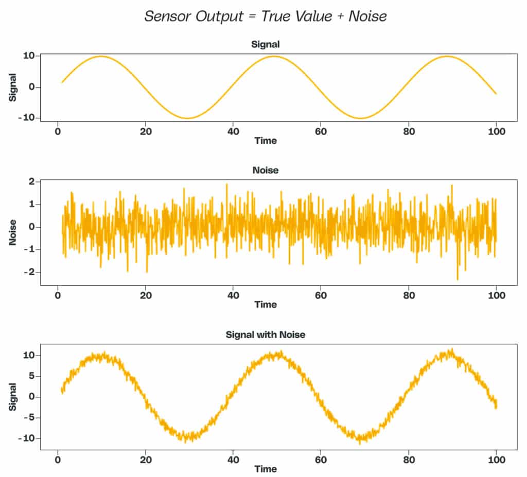
Noise comes from various sources ranging from the environment to internal electronic components (thermodynamic and quantum effects). We can quantify and mathematically remove some types of noise from the sensor output. Unfortunately, other types of noise defy quantification and need to be handled with other methods that don’t require as much knowledge about the data. Before we can use sensor data in machine learning algorithms, we must understand some important aspects of the sensors as well as the sampling to pre-process the data.
This is where signal processing – analysis and modification of measurements from instrumentation – comes in to help us pre-process the data before we feed it into an ML model.
Signal processing is a branch of electrical engineering that deals with the analysis and modification of measurements collected from the instrumentation.
Finding a Signal in the Noise
In most cases, the average strength of noise (N) will remain constant and independent of the signal (S). The effect of noise on the error of the measurement will be greater when the quantity to measure decreases in magnitude. Accordingly, the signal (S) to noise (N) ratio can be written as:

As a basic metric, if the signal-to-noise ratio is below three, it is impossible to detect a signal.
Types of Noise in a Typical Production Environment
Instrumental Noise
Noise arises from every part of a sensor, starting with the sampling method, source, internal electronics (transducers and circuitry), and signal processing aspects. Thermal, shot, and flicker noise are some of the most common forms of instrument noise.
Thermal Noise
Sensors contain many electrical components which electrons pass through. These components include resistors, capacitors, transducers, and other resistive elements. As electrons move through these elements, they generate heat and voltage fluctuations. The voltage fluctuations display as noise in the sensor. We can quantify this noise as:

where the root mean square noise voltage (v) is equal to the square root product of Boltzmann’s constant, Temperature, Resistance, and frequency bandwidth.
Shot Noise
Shot noise arises from fluctuations in DC current because electrical current is composed of discrete components — electrons. Shot noise usually dominates at high frequencies and low temperatures.
Flicker Noise
Flicker noise is often referred to as pink noise and is present in low frequency applications as opposed to white noise, which is found in higher frequency applications. Flicker noise has a magnitude that is inversely proportional to the frequency of the signal. While flicker noise is ubiquitous in low frequency applications, its effect can be reduced by using wire-wound or metallic film within the sensor circuitry.
Environmental Noise
Environmental noise refers to all the various sources of interference present in the same environment as the sensor. For example, if there are sources of vibration from heavy machinery in an environment, this may have an impact on sensors that are sensitive to that specific noise. Additionally, a sensor and its components can act as an antenna for electromagnetic radiation that can be caused by lines of AC current, electrical motor brushes, lighting, and radio frequencies, among others.
Analyzing Noise
Choosing the Optimal Approach to Sampling Frequency
Sampling frequency [represented in Hertz (Hz)] is the number of samples obtained in one second. It’s important to understand the nuances of sampling frequency for proper filter design, and application of both standard and advanced noise analysis techniques.
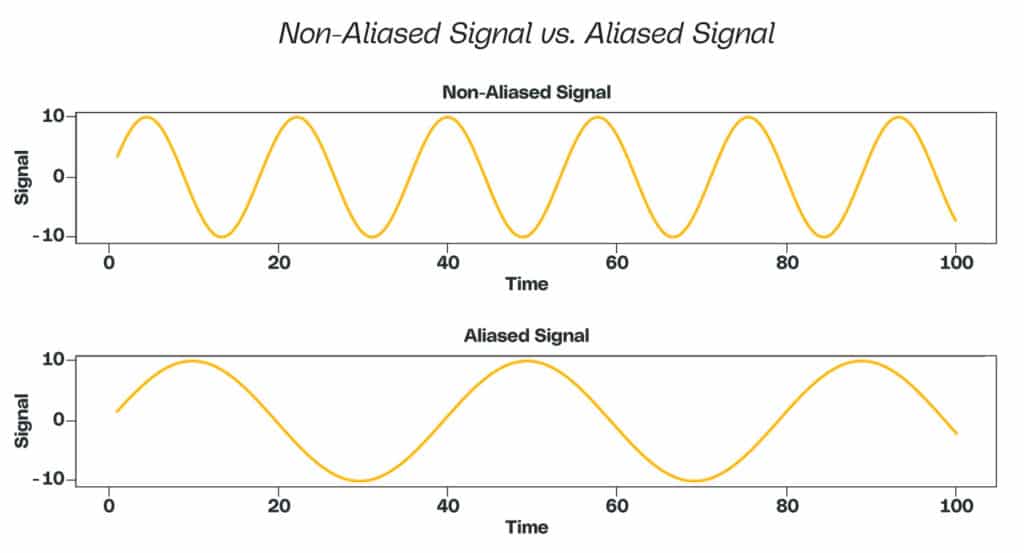
When dealing with pre-built sensors, we usually optimize sampling frequency to eliminate a phenomenon called aliasing. Aliasing occurs when a signal is sampled too slowly, and as a result, certain amplitudes may be missed. It is always good to clearly identify what we’re trying to measure and understand the capabilities of the measuring device. We may wish to sample at a lower frequency to consume less power and decrease the payload of data from the sensor. Even though the end use may not require a high frequency, it is best to oversample until we discover the appropriate frequency. We can downsample high frequency signals later, but upsampling will be difficult, if not impossible, and we will lose important values.
Dashboarding
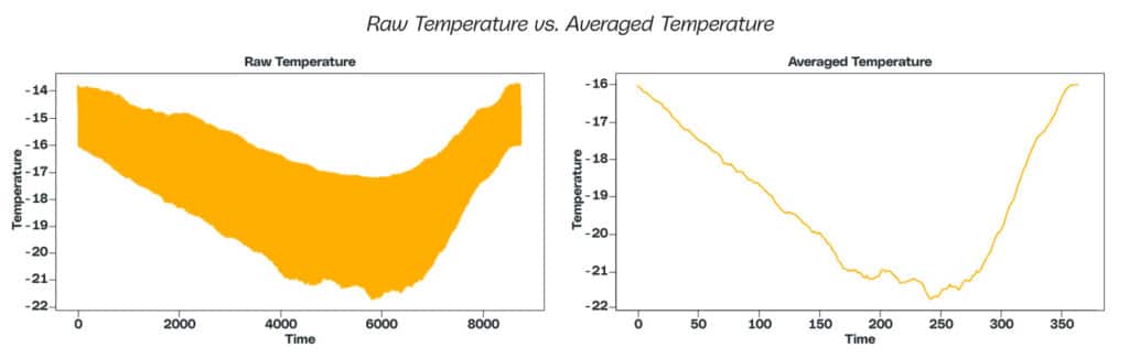
Sensor frequency is also an important topic when it comes to data visualization and dashboarding. Sensors sample multiple times per second. While this information may be useful for an algorithmic use case, it may not be beneficial for visualization. For visualization, downsampling or averaging to a higher time interval results in more legible outputs. For example, you can see a raw signal on the left versus the averaged signal on the right. Simplifying the outputs makes them easier for operators or analysts to gauge sensor output over time and establish a general idea of the measurements taking place.
Filters
A staple of signal processing is the application of filters. Filters work in both analog and digital applications to accomplish similar tasks. Filters come in different types such as a low-pass filter, high-pass filter, and band-pass filter, to name a few. These filters work by passing a signal above (low-pass), below (high-pass), or between (band-pass) a certain cutoff frequency and attenuating the signal that does not meet the specified criteria. These types of filters work very well where there is a constant and consistent source of noise. In addition, these filters are easy to implement. We can integrate them into hardware as part of the internal circuitry of a sensor and apply them digitally as an edge compute case or as a treatment to the raw sensor output.
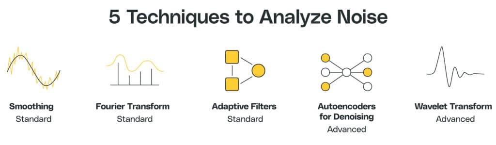
Standard Techniques
Smoothing
When dealing with sensor data, smoothing is a good first step. This step is crucial because any other transforms done to the data for feature extraction and engineering may increase noise if the data is not smoothed first. Smoothing also helps eliminate high-frequency noise, which in turn will affect transforms and downstream modeling methods. The Savitzky-Golay smoothing filter is a robust smoothing method that can be applied to a host of sensor data, both in one and two dimensions.
The Savitzky-Golay smoothing filter works by first selecting and optimizing two parameters — the window size and the degree of polynomial. Using this information, the filter fits the degree polynomial to the specified window size and the smoothed data is used as the output. There are several methods to optimize the window size and polynomial degree that can be utilized. This method works well for a variety of applications and serves as a foundational tool for pre-processing sensor data.
Fourier Transform
Simply put, the Fourier Transform tells us all of the different components that make up a signal. This transform works best for stationary signals — those that maintain the same frequency over time. For example, the Fourier Transform would be useful to control noise from a sensor near multiple pieces of machinery that cause unwanted vibrations which are constant over time. The Fourier Transform is one of the most commonly used transformations in signal processing because it allows signals to be viewed in a different domain, specifically the frequency domain instead of the time domain. This will show what frequencies are present in the signal as well as their proportions.
When it comes to noise from one or many sources, the Fourier Transform enables us to identify and nullify problematic frequencies. There are also techniques and theorems built on top of the Fourier Transform that we can use to measure the energy of the signal as well as perform convolutions.

The Fourier Transform is a very common technique for signal processing. However, one main disadvantage of the Fourier Transform is its inability to capture local frequency information. The Fourier Transform captures frequencies that persist over an entire signal. We can overcome this limitation by using a Wavelet Transform.
Adaptive Filters
Adaptive filters contain two components: a linear filter and an adaptive algorithm. The adaptive algorithm changes the parameters of the linear filter to minimize the signal error. Adaptive filters are useful because they allow us to remove noise that changes over time. In an industrial setting, this can be very useful to handle environmental noise that may be changing and non-constant.
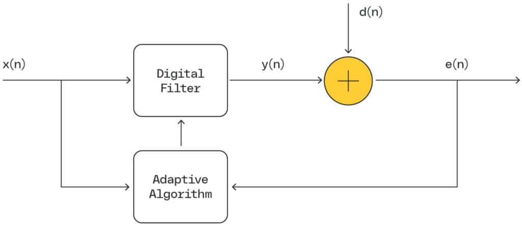
The adaptive filter works by having an adaptive algorithm adjust the weights of the digital filter. A reference input signal x(n) is passed through the filter to provide an output signal denoted as y(n). A desired signal d(n) is compared against the output signal y(n) to produce error, e(n). The adaptive algorithm adjusts the filter weights to minimize the value of e(n).
While adaptive filters are useful, they shouldn’t be used if the noise in an environment is constant. If it is constant, then there are computationally less expensive filters (like band-pass filters) that can be used. An understanding of signal and noise is also important to determine the adaptive algorithm to use — Gaussian versus non-linear. For example, if the output data contains noise that is not proportional to the signal, then we would apply a non-linear adaptive filter algorithm.
Advanced Techniques
While we prefer the above standard techniques where possible for their simplicity and relative computational efficiency, they’re not right for every situation. In industrial settings, there may be multiple and compounding effects of noise. When noise is complex, using multiple filters or steps to denoise may not be suitable. Multiple steps will increase latency in reporting data as well as compute power and resources — especially if it is being computed on the edge.
Autoencoders for Denoising
One approach to denoising complex noise patterns is to use a denoising autoencoder (DAE). A DAE is a machine learning algorithm that has the capability to provide robust denoising, especially when the sources of noise are not well understood and cannot be filtered out effectively with standard tools. DAEs can be quantized, which means that a large model such as a neural network can be modified so that it can perform its function on an edge compute device. An autoencoder is a neural network with the following type of architecture:
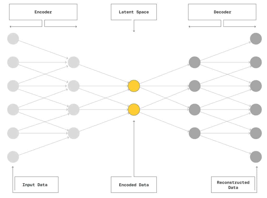
The DAE seeks to take noisy data as an input and discover its latent structure. The network consists of an encoder and a decoder. The first half of the network is the encoder, which transforms the noisy input into its latent structure at the bottleneck layer. The second half of the network is the decoder, which reconstructs the input data using the latent representation. The final output is a reconstructed signal that has been denoised.
Mathematically this is represented by equation 1 as the encoder, which maps input x to z using a nonlinear activation function denoted as f.

In equation 2, the decoder maps z to x which is the reconstructed version of the input using g, a nonlinear activation function. W and b represent the weight and bias matrices.

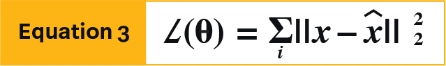
Finally, the objective function of the autoencoder is represented by equation 3, which seeks to minimize the error between input and output using an absolute square difference.
Wavelet Transform
Some signals that have oscillations of short duration may not be well suited for a Fourier Transform. The Wavelet Transform improves on the Fourier Transform by decomposing a signal into a set of wave-like oscillations localized in time.
The Wavelet Transform selects a wavelet shape and slides the shape over the signal. At each timestep, the wavelet is multiplied by the signal and the resulting output provides a coefficient of the wavelet scale. This approach extracts both local temporal and spectral information at the same time. It is a more efficient approach than using the Short-Time Fourier Transform.
The Wavelet Transform represents a very useful method for short oscillations and non-stationary signals and provides a reliable method for other tasks in signal processing, such as correcting baseline drifts in signals.
Use a continuous Wavelet Transform to analyze the entire signal by letting both the translation and scale parameters vary continuously.

Use a discrete Wavelet Transform to capture both the frequency and the location (in time) information.

The continuous Wavelet Transform works best for time series data because it can set the parameters for scale and position, which results in higher resolution. The discrete wavelet transform decomposes a signal into different sets and is most useful for feature engineering or data compression.
Deploying Your Models
We can deploy signal processing at different stages in the data acquisition process. It all depends on understanding the process and the impact that the data has on downstream processes. For example, if we need sensor data as part of a feedforward or feedback control system, we need to apply a lower latency version of signal processing. In this case, the best option would be an edge compute application, where we program the filter into the sensor at a hardware level. If, however, we use signal processing for data analysis and understanding trends over time, we may wish to deploy the model at a local terminal where the analysis is taking place or have it be a part of a data pre-treatment process in a historian database.
What To Do With the Discovered Signals
Once we pre-process a signal, we can do many things with it. We can use signals to help control and optimize processes through feedback and feedforward control loops. We may also choose to develop a machine learning model for process optimization and predictive maintenance, visualization, monitoring, and alerting.